Introduction
Data augmentation — is a powerful regularization technique for object detectors, as well as for any model, working with visual data. In addition, data augmentation helps to artificially enlarge datasets, if you do not have enough instances in your training dataset.
However, before you find a proper augmentation technique, it is crucial to visualize the data augmentation pipeline. Moreover, some Tensorflow functions have a large variety of parameters, which leaves ML engineers confused about their correct use.
Therefore, this article visualizes the main data augmentation techniques for Tensorflow object detection models, and describes the meaning of each function parameter.
After reading this article, you will understand:
-
How 10 out of 36 image augmentation techniques modify images in Tensorflow object detection
-
Which transformations will increase performance of your image recognition model
Moving through the paper, we will cover 10 of the 39 available data augmentation functions, described in the Tensorflow preprocessor.py file. A part, dedicated to each function, is split into several subsections:
-
Before / After — illustration of the data augmentation function, with an explanation of the performed modification.
-
Separate series — a result of applying data augmentation to the image several times (which, due to the probabilistic algorithms, will provide different images). This section will allow you to understand, how your image will be modified and presented to models in different mini-batches.
-
Function parameters explanation — because some of the functions have up to 7–8 parameters, which can confuse users. It is primary to understand the meaning of every parameter. Some of them can lead to skipping-out classes out of the image (e.g. random cropping, which we will discuss in the article)!
P.S. For all images, that you will see below — the original photo can be found via this link.
Let’s get it started!
Random horizontal flip, Random vertical flip
In preprocessor.py: random_horizontal_flip, random_vertical_flip
Before / After
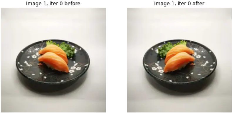
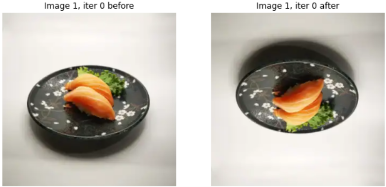
In the image below, we can see that this function randomly rotates the image around its vertical axis (for a horizontal flip). Vertical flip does a similar transformation, rotating the image with respect to another axis.
Separate series
As an image is encountered from minibatch to minibatch, it will be rotated with a certain probability. Probability is a parameter of applying this augmentation function.

Function parameters explanation
This function has only one parameter — probability, which determined how likely the image is rotated, during the data augmentation step. Preferably, for a probability = 0.5, your model will be presented with equal shares of the original and flipped images.
Random adjust brightness
In preprocessor.py: random_adjust_brightness
Before / After
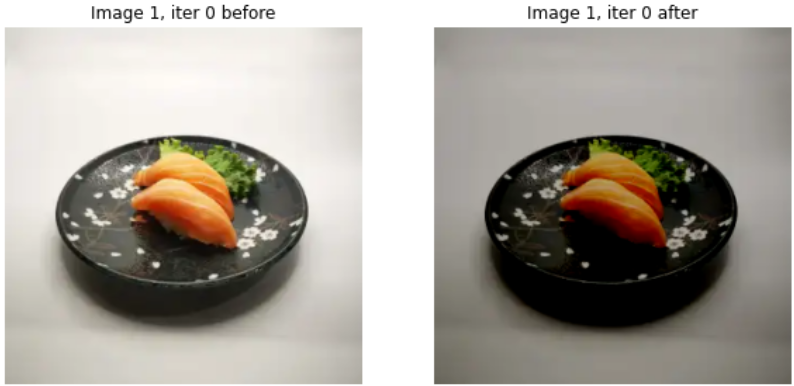
The functions algorithm is the following:
- Randomly generate delta from range (
-max_delta,+max_delta), wheremax_delta— parameter of the function (remember,max_deltamust be from 0 to 1. On the image above,max_delta = 0.5) - Downscale image by dividing it pixelwise on 255
- Add delta to all components of the downscaled image
- Upscale resulting image by multiplying it pixelwise by 255
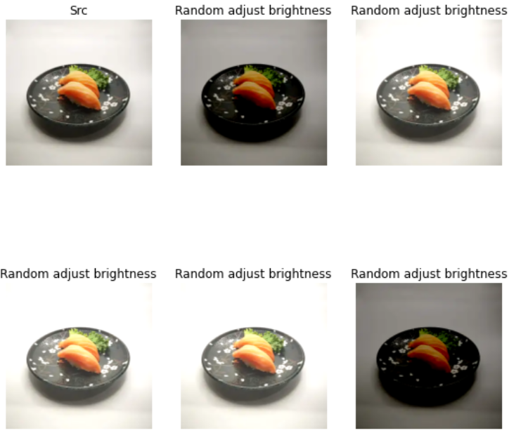
Remember, that this data augmentation can both darken and lighten images! Therefore, it is useful, if your object detector is subject to varied lighting conditions for images.
Separate series
The image below demonstrates, how your model will see augmented image through several mini-batches (if the same image is sampled into some of them).
Function parameters explanation
The function has two parameters — seed and max_delta.
seed — is necessary for reproducible results.
max_delta — regulates, how much is added (subtracted) from the image, downscaled to the pixel range [0.0, 1.0]. Beware, max_delta cannot surpass (0.0, 1.0) range!
Random black patches
In preprocessor.py: random_black_patches
Before / After
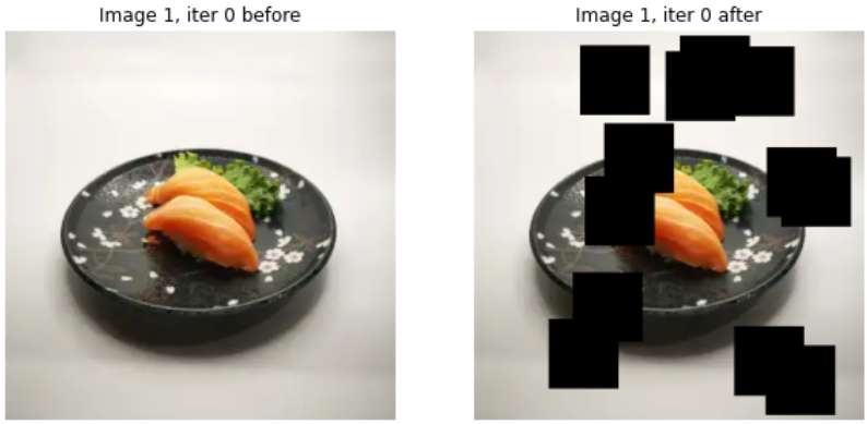
As you observe in the image below, this augmentation is crucial for object detection tasks, when an object is particularly overlapped. Random black patches force a model to recognize an instance by its parts. For example, in this image, a model will be forced to detect sushi, based on their right halves and the presence of fish on top. As well, the plate will not be entirely visible during the whole training process.
Separate series
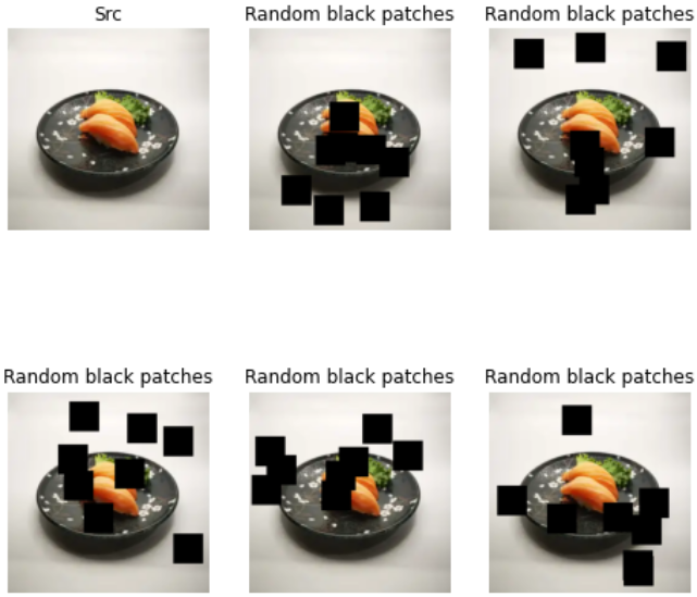
An image below shows you, how it will be presented to the object detector, after applying black patch augmentation. Here, you can make several important notes:
Your target classes (e.g. sushi on the image) will not be covered every time! The patches are applied probabilistically, and the chance of covering your target object depends on the patch size, number of patches, and probability of patches. Luckily, they are the parameters of the function.
Function parameters explanation
-
random_seed— we needrandom_seedfor reproducible results. -
max_black_patches— how many times the function tries to add a patch to the image. Every try, a patch is added with a certain probability (regulated by the probability function parameter). -
size_to_image_ratio— determines the patch size. According to documentation, patch size is determined by the equation below:patch_size = \ size_to_image_ratio * min(image_width, image_height)
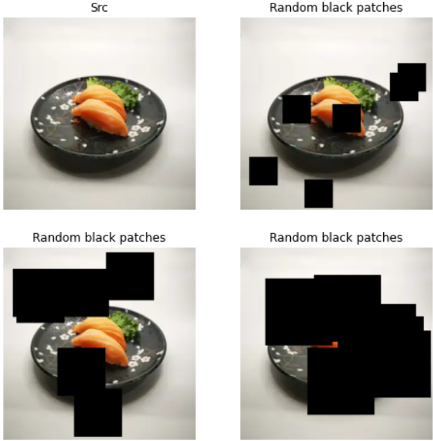
For example, below you will see a visualization of 8 black patches, applied to the image with 90% probability, with different size_to_image_ratio parameters: 0.15, 0.25, and 0.25 respectively. Important conclusion: you must carefully choose the function parameters and visualize their effect! As you see, it can black out your target classes!
Random patch Gaussian
In preprocessor.py: random_patch_gaussian
Before / After
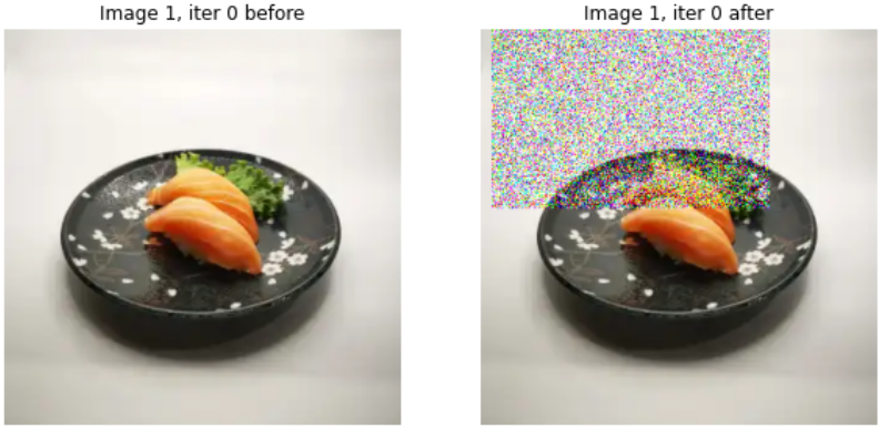
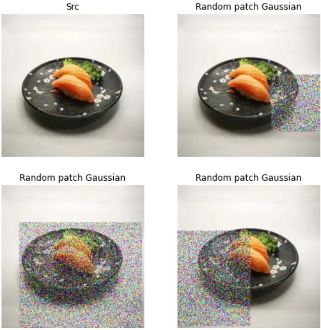
The functionality of Gaussian patches is very similar to the black patches, that we have discussed previously. Adding random noise to images sometimes helps to regularise models, preventing them from overfitting to particular pixels.
The Gaussian patch algorithm is the following:
- Scaling image by pixelwise division by 255.0
- Adding gaussian noise to the scaled image
- Clipping result, to comply with [0, 1] range for each pixel value
- Scaling image back to [0, 255] range by multiplication
Separate series
Pay attention that, due to probabilistic augmentation, your patches will not always be covering your target classes!
Function parameters explanation
-
min_patch_size,max_patch_size— integers, that define the minimum and maximum size of patches. Resulting size is a randomly sampled number from [min_path_size,max_patch_size]. -
min_gaussian_stddev,max_gaussian_stddev— floats, that define the minimum and maximum standard deviation of the noise, that will be applied to the image (in the patch region). Standard deviation for current iteration will be randomly samples from [min_gaussian_stddev,max_gaussian_stddev]. -
random_coef— the probability of returning the original image. Ifrandom_coefis 0, a patch will be applied with 100% probability. -
seed— for reproducible results.
Random crop image
In preprocessor.py: random_crop_image
Before / After
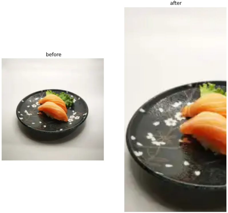
Random cropping — is a process of cropping out a subset of the image. Beware, that random cropping modifies image size, the resulting crop is smaller! It can lead to cropping-out target classes out of the image, as we will see.
According to the documentation:
- The algorithm tries to sample a crop window, compliant with user constraints (defined by function parameters)
- If within 100 trials cropping is unsuccessful — the original image is returned! If you set too demanding constraints — you will not augment your dataset!
Separate series
Random image cropping – is one of the most dangerous data augmentations. In the images below, you can understand why.
First and foremost, we label the photo with two instances of sushi and one instance of the plate. Note, that the photo contains two small classes, and one large (plate), which “wraps” the smaller ones. This is the key to understanding the danger of cropping.
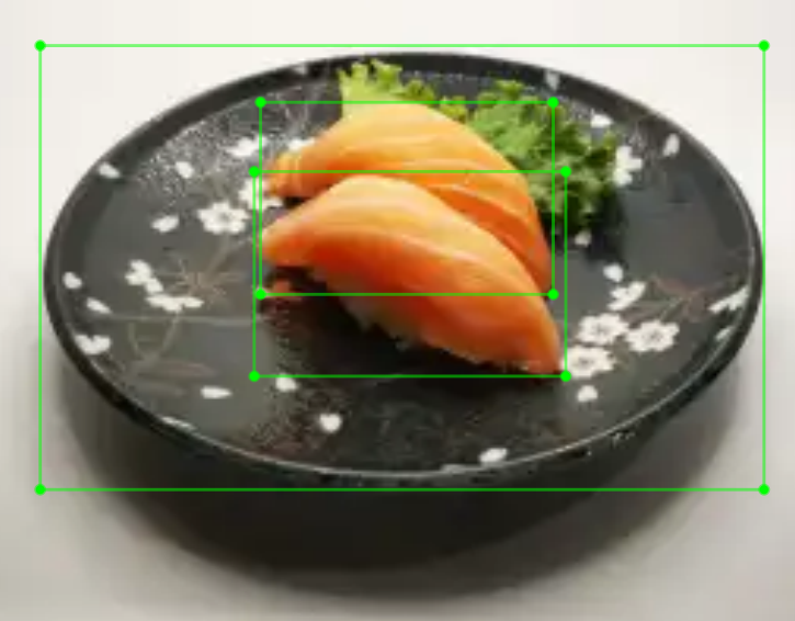
For this series of images, the user constraints were:
min_object_covered: 0.1 (As a minimum, cover 10% of the whole object)aspect_ratio_range: (1, 1) (Allowed range of aspect ratio for cropped image)area_range: (0.01, 1.0) (Allowed area range for the cropped image)overlap_thresh: 0.3 (If overlap with the bounding box is less than 30%, the algorithm deletes this bounding box!)
Below you see the result of applying random_crop_image function with the above parameters. In some mini-batches, the cropping augmentation crops out smaller classes!
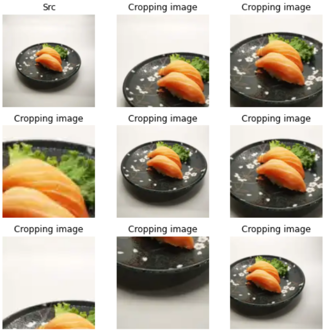
Cropping out your target classes during training could be critical for your object detection task, if you have an extremely small dataset, and do not want your model to miss out on labelled data. Think twice and visualize carefully chosen parameters, before you decide to apply this function in your data augmentation pipeline. And remember, that this function modifies image size, which might not be desirable for your task.
Function parameters explanation
-
min_object_covered— the cropped image covers at least themin_object_coveredpercentage of at least one object on the image. It means, that if the function coversmin_object_coveredof one class — it can crop the image, to exclude all other classes. An example of excluding classes is on the image above — when the cropping covers 30% of the plate (but not sushi) — it selects the crop, where sushi is not presented! -
aspect_ratio_range— tuple of two integers or floats. The aspect ratio will be chosen randomly from the range(aspect_ratio_range[0],aspect_ratio_range[1]). Regulates the aspect ratio of the cropped image. For example, on image below for several values ofaspect_ratio_range— (1, 2), (2, 3), and (0.1, 0.2) respectively.
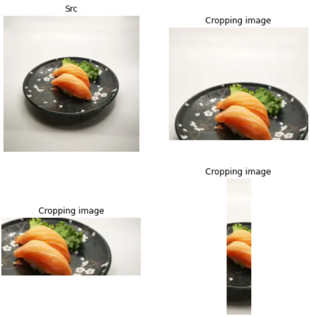
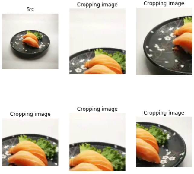
area_range— allowed range of area(cropped_image) / area(source_image). On the image below, you can see variations of croppings, performed for the samearea_range = (0.1, 0.2)
-
overlap_thresh— If the bounding box overlaps with cropped image by less thanoverlap_threshpercent — the algorithm will delete this bounding box. This is dangerous because you can skip your target classes. Be aware when regulating this parameter. -
clip_boxes— If the bounding boxes are “clipped” to the new, cropped image. By default, this argument isTrue, and we recommend keeping itTrueunless the task is very specific. If you do not clip your bounding boxes to new image dimensions — you will have negative bounding box coordinates. Because old coordinates are no longer present on the cropped, smaller version of the image, they will turn into negative values. -
random_coef— the probability of returning the original input image. Whenrandom_coefis set to 0.0, the algorithm will always modify the image (which is something you might not wish for, as the model should be presented original data sometimes). -
seed— for reproducible results.
Random jitter bboxes
In preprocessor.py: random_jitter_boxes
Before / After
We skip the Before / After section, because this is not an image augmentation technique. However, you will see what it does with bounding boxes on the images below.
Separate series
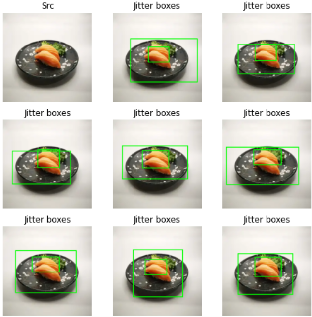
As you see, box jittering — is a process of “shaking” your bounding boxes. This technique is useful, if you are not sure about the quality of labeling, and want to make your model robust to less precise tagging. However, beware the danger of using this technique, because sometimes, when a model gives precise detections, jittered ground truth forces the model to shift the predicted bounding box and make it less accurate.
Function parameters explanation
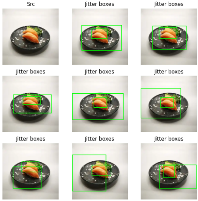
ratio— for example, if the bounding box is 100 pixels in linear size, and theratiois 0.05 — then the corners of the box can jitter up to 5 pixels. For instance, below you can see separate images for various values ofratioparameter: [0.1, 0.2, 0.3, 0.4, 0.5, 0.6, 0.7, 0.8]. It means, that in the last photo, the bounding box could fluctuate 80% of the bounding box size. As you see, the higher theratiois, the more severe the regularization. Up to the point, that a model will not be able to learn if the boxes are jittering too much.
-
jitter_mode— various modes of jittering, described below (cited from documentation):- expand — only expands boxes
- shrink — only shrinks the boxes
- expand_symmetric — expands the boxes symmetrically along height and width, without changing the box center. The ratios of expansion along X, and Y dimensions are independent
- shrink_symmetric — same as above, but shrinkage
- expand_symmetric_xy — expands the boxes symmetrically along height and width dimensions. The ratio is no longer independent for x and y — now it is the same for both
- shrink_symmetric_xy — Same as above, but shrinkage
- default — Randomly and independently perturbs each box boundary
-
seed— for reproducible results.
Random pad image
In preprocessor.py: random_pad_image
Before / After
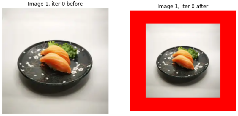
As you can see below, random padding adds default vertical and horizontal margins to the image. Keep in mind, that this augmentation modifies image size. The function works in the following way:
- First, a padded, enlarged picture of default values is created
- The image is located uniformly, at a random location of the padded default “wrapper”
Separate series
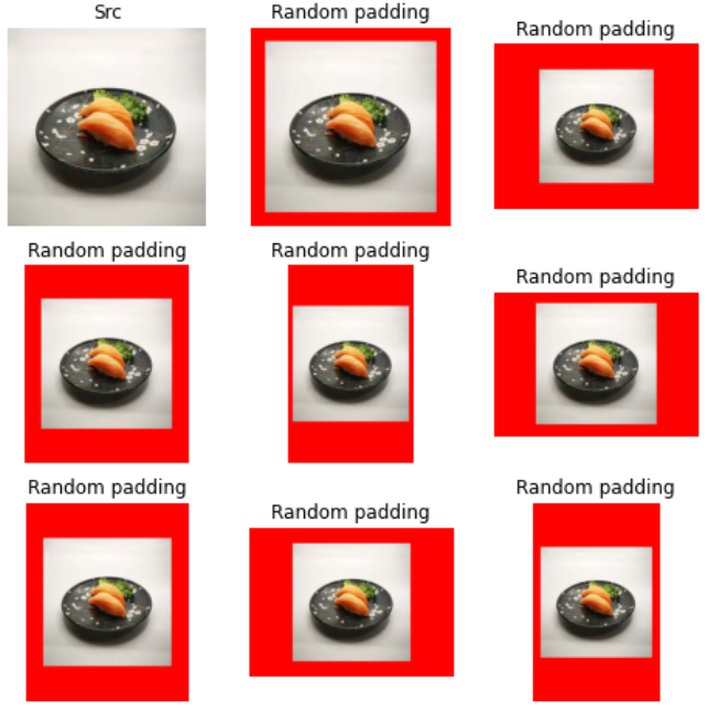
In the following picture, notice how greatly vary the linear sizes of the resulting image. Even though they seem the same, images’ linear sizes vary from 300 to 500 pixels.
Function parameters explanation
-
min_image_size— a tensor, consisting of two values. For each iteration, the minimum image size will be sampled at random from your specified range. For example, if you want the minimum size to be always above 350 pixels, but never exceed 500, initialize this parameter as follows:min_image_size = \ tf.constant([350, 500], dtype=tf.int32) -
max_image_size— parameter, that describes the available range for maximum image size in pixels. Initialize it the same way asmin_image_size. -
pad_color— the color of padding in RGB color scheme. Initialize this parameter as shown below:# for red color pad_color = \ tf.constant([255, 0, 0], dtype=tf.float32) -
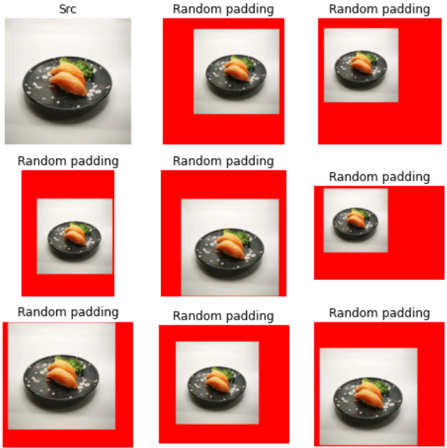
pad_center— defined, if the original image will be placed in the center of the padded rectangle, or not. For instance, in the picture below you will see paddings, forpad_center=False:
Random adjust contrast
In preprocessor.py: random_adjust_contrast
Before / After
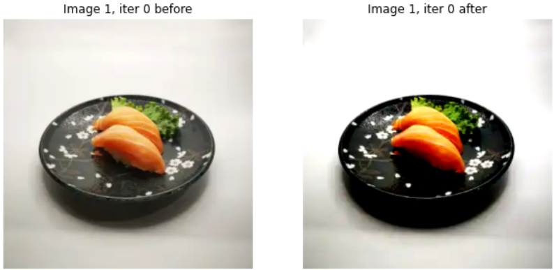
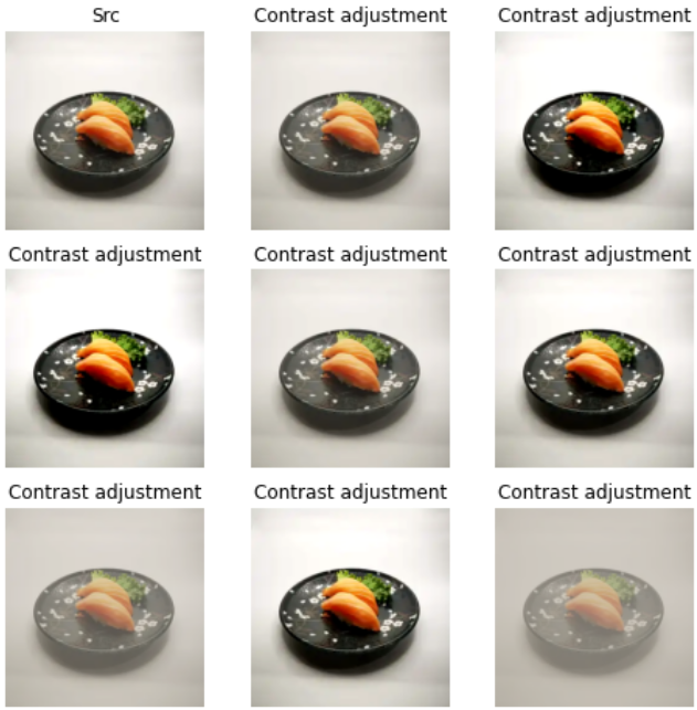
A function explains itself — it adjusts the contrast of the image. However, if contrast distortions are not typical for your task domain — it might not be reasonable to include this technique in your augmentation pipeline.
Separate series
Beware, that, as the image below suggests, random contrast adjustment can both enhance and weaken the contrast of your train images! As your image will be presented across several mini batches — its contrast will be both enlarged and suppressed.
Function parameters explanation
-
min_delta,max_delta— floats, that regulate the magnitude of contrast adjustment. For reference, in the series of image above,min_delta = 0.3,max_delta = 1.6. -
seed— for reproducible results.
Random adjust hue
In preprocessor.py: random_adjust_hue
Before / After
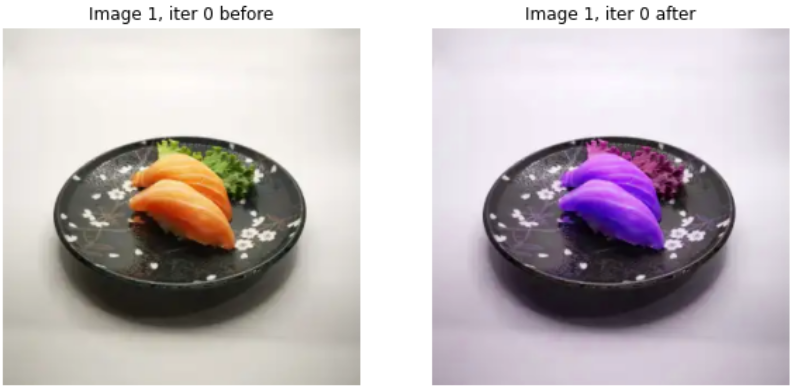
This preprocessing is reasonable if your images are subject to hue and color distortions, that affect the whole image. Otherwise, consider not taking advantage of this technique, as it might worsen your model’s performance.
Separate series
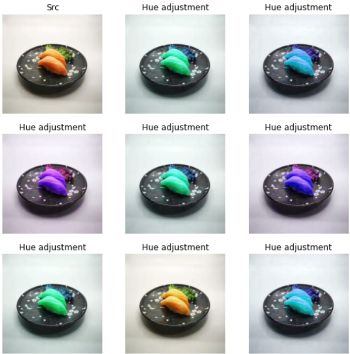
Down this text, you see how significantly it distorts the color of the image. Be mindful of embedding this technique into your augmentation pipeline. It might not be reasonable for food-related tasks, as the color change is not so critical.
Function parameters explanation
-
max_delta— the intensity of the hue modification. For reference,max_delta = 0.5on the image above, which already leads to intense distortion. -
seed— for reproducible results.
Conclusion
Good job! In this article, we have covered 10 data augmentation techniques, available in Tensorflow object detection framework. Let us highlight how important this is to visualize your data augmentation pipeline, with the selected hyperparameters.
Today, we have seen that some functions are probable to crop out your target classes, blackout them, or even delete or shift your bounding boxes! This is primary to understand, before taking advantage of image data augmentation. The key takeaways of the article are:
- Random black patches data augmentation can black out your target classes from the image. If the patch size is large, it will overlap with the target class on the image. You have to use this technique mindfully and experiment with the size and probability of the patches.
- Random cropping is a dangerous data augmentation technique since it can crop out your target classes of the image. You must carefully choose the parameters of the random_crop_image data augmentation function.
- Data augmentation is a powerful regularization technique, that allows you to reduce the variance of the model, preventing it from overfitting on your training dataset, and increasing the model’s generalization ability.