Introduction
Hello there!
This article is devoted to my project, available on github. We will use popular CNN architectures to estimate crowd numerosity in a busy shopping mall. This problem originates from a Kaggle discussion, dedicated to crowd detection.
We will cover following topics:
-
Alternative approaches to crowd counting, and why Deep Learning is an effective method as well
-
Famous “Shopping Mall” dataset
-
Experiments, performed with six popular CNN architectures, to approach a crowd numerosity estimation
-
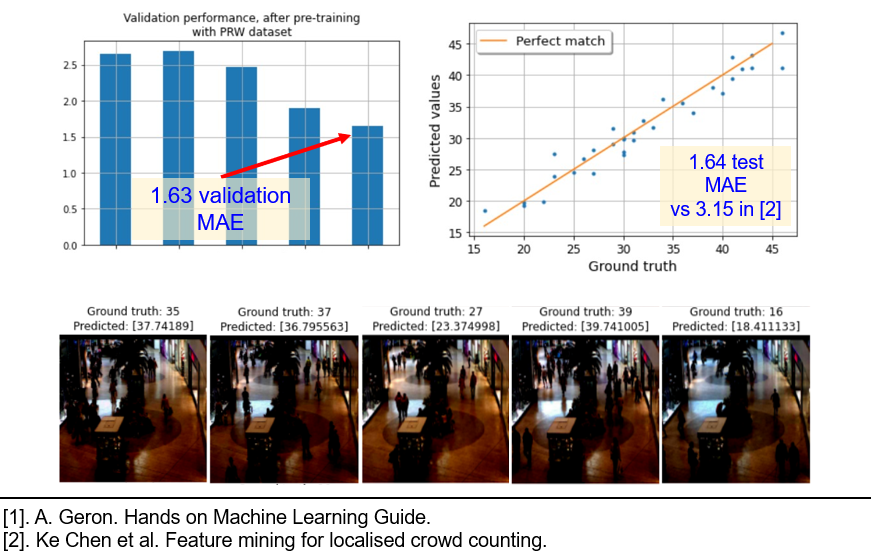
Results of the best model on the test set, and concluding with the most efficient transfer learning techniques, that helped to achieve 1.64 MAE test performance
Alternative approaches to crowd counting
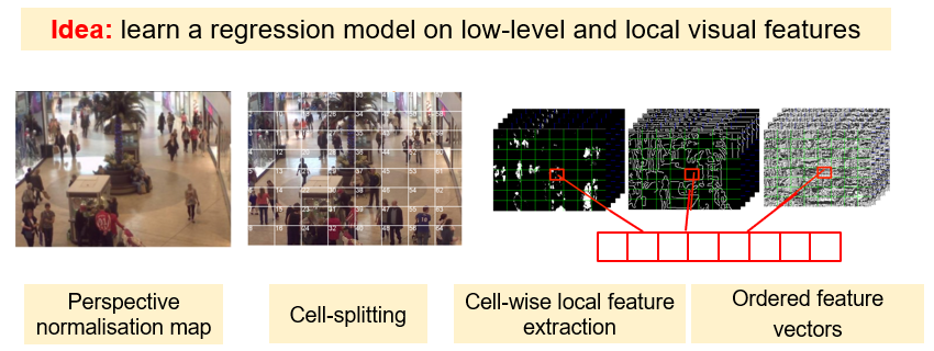
Alternative approaches are divided into regression-based, detection-based, and clustering-based. Regression-based methods use the key idea of extracting local visual features. For this techniques, the features, extracted from the raw image, represent an input to a regression model, predicting the crowdedness.
For example, the work of Chen et al. splits an original image into a grid of cells. From each cell, local visual features are extracted. In summary, each input image is transformed into a cell-ordered numerical vector, that encodes the extracted features. This vector represents an input for a multi-output regression model, predicting number of pedestrians in each cell independently. Such approach achieves 3.15 Mean Absolute Error (MAE) on a “Shopping Mall Dataset”.
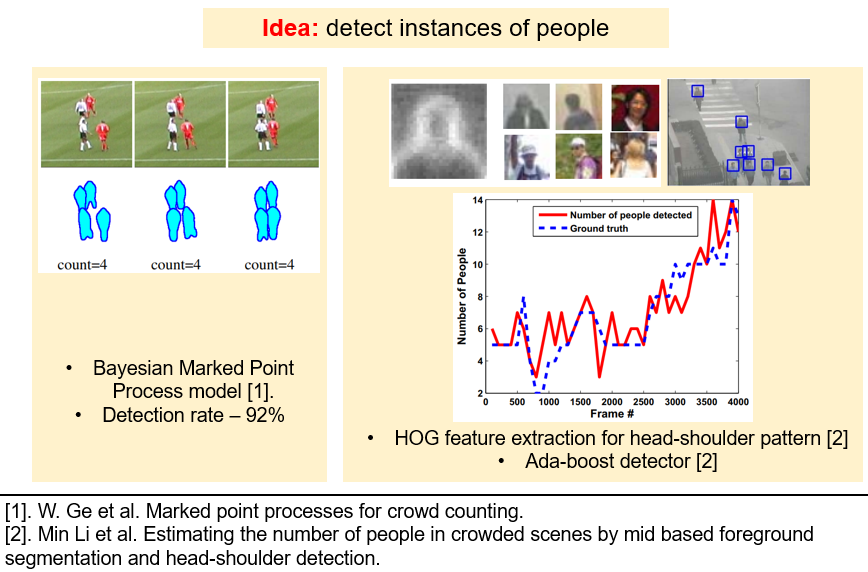
The researchers, who follow the detection-based approach, use the models of classic Machine Learning, or Deep Learning, or even probabilistic models, to detect instances of people. As you see in the picture below, W. Ge et al. uses Bayesian algorithms to detect players on the field, while in the paper of Min Li et al., an adaboost regressor detects the head-shoulder visual patterns, that are robust to crowdedness and occlusions.
Such models perform at a fairly high detection rate of 92%, and the predicted crowd numerosity is visually close to the ground truth (as it follows from the plot below).
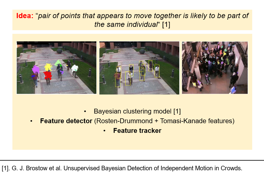
The concept of clustering-based approach is that a moving human represents a “cloud” of points, moving coherently. Thus, one can take advantage of clustering methods, to detect such regularities. The inference pipeline consists of a feature extractor, and a clustering algorithm, analyzing the sequence of video frames, and taking the extracted visual features as an input (like in the work of Brostow et al.).
The advantage of the deep learning approach is in having a single model, responsible for both feature extraction and prediction. Many pipelines in computer vision rely on local visual features as input. These features depend on the feature extractors (e.g. Histogram Oriented Gradients, foreground extraction, edge detectors), that are selected by the creators of the pipeline. Convolutional Neural Networks, instead, are capable of automatic “customization” of the feature detectors, to make them suitable for a particular dataset. This enables an “end-to-end” learning system, when developers do not waste time on finding suitable feature extractors. We will focus on the deep learning approach. Moreover, to enhance the performance, we take advantage of transfer learning techniques.
Dataset
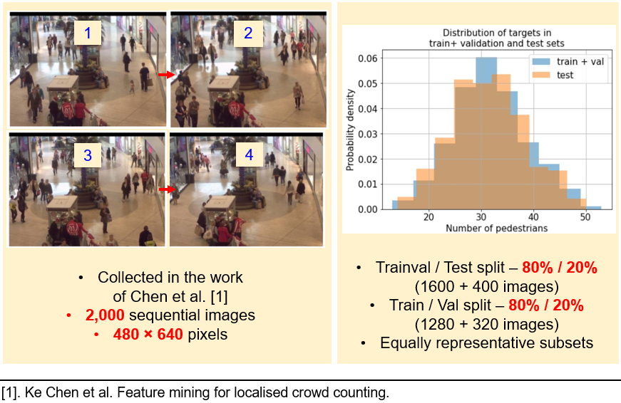
As you see from the image below, a dataset represents 2,000 sequential images of people, walking in a busy mall. The dataset was split into trainval and test sets, with 80% and 20% proportions. On the histograms below, it is controlled, that the test and trainval data comes from the same target distribution (target is the number of people in the image). Then, the trainval data is randomly split into train and validation sets, in proportions of 80% and 20%.
Experimental scheme
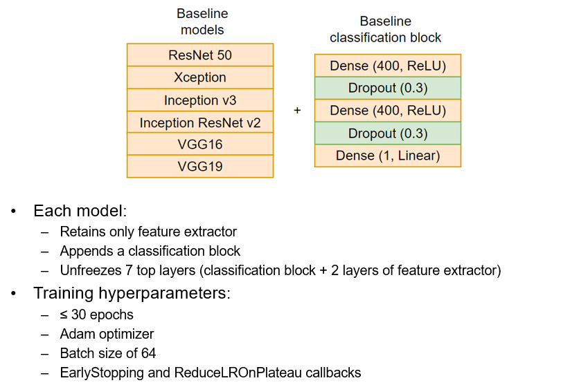
We start with training six popular CNN models – ResNet50, Xception, Inception v3, Inception ResNet v2, VGG16 and VGG19. For each architecture, we maintain the same training hyperparameters, to compare, how these models behave at the baseline level. Moreover, for each model, we retain the feature extractor part, that was pretrained on ImageNet dataset. The selection of the best baseline depends on several criteria:
- Smoothness of the learning curve
- Training time (per epoch)
- Number of trainable parameters
- MAE error on validation dataset
Then, the best baseline is improved with several transfer learning techniques:
- Pretraining with additional dataset
- Selecting the optimal number of unfrozen layers
- Using the pre-training technique, cited from the book of
A. Geron “Hands-On Machine Learning Guide”.

The feature extractors of each models were appended with the classification block, consisting of ReLU and fully connected layers. As you see in the picture below, all models share the same training hyperparameters (number of epochs, optimizer, batch size, and callbacks).
Experimental results
After defining the experimental scheme, we are ready to perform the computations and report the results!
The best baseline model
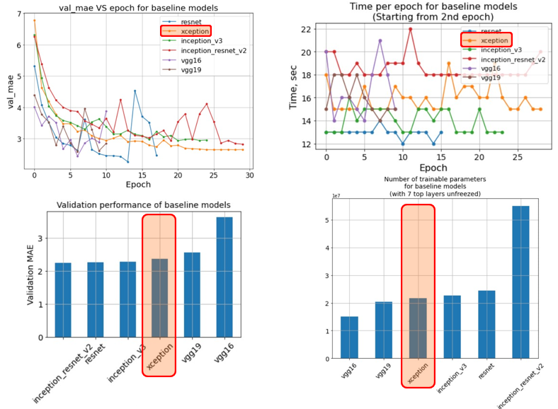
In the image below, the baseline models were compared, according to four main criteria. From these plots, we can make several conclusions:
-
The learning curves fluctuate, which suggests decreasing the learning rate and the batch size. These suggestions are accounted in the subsequent part of the work
-
Resnet 50 and VGG19 models are characterized with the steepest decline of the learning curve, which indicates better learning capacity
-
According to the plots, the Xception architecture is a “golden middle”, that has a smooth learning curve, moderate training time per epoch, and achieves 2.3 validation MAE error, while having moderate number of trainable parameters
Therefore, we select Xception architecture for further experiments! Now, we will apply transfer learning techniques, to boost the performance of the Xception model.
The best number of unfrozen layers
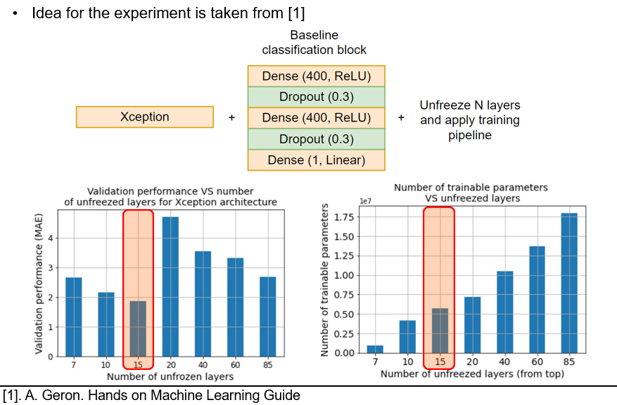
The idea for this experiment is cited from the book of Aurelien Geron. To maximize the performance of the transfer-learned model, one must find the best number of unfrozen layers.
In our experiments, the 15 unfrozen layers yield the lowest validation MAE error, while do not result in a large number of trainable parameters. Therefore, for the next experiments, we unfreeze 15 layers from the top. Beware, that the number of the unfrozen layers should change accordingly, if you decide to deepen the classification block of your model.
Pretraining with a new dataset
The images below represent a PRW (Person Re-identification in the Wild) dataset, first introduced in the work of Liang Zheng et al. The dataset consists of 11,816 sequential images, shot near the Tsing Hua University.
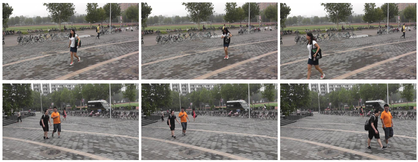
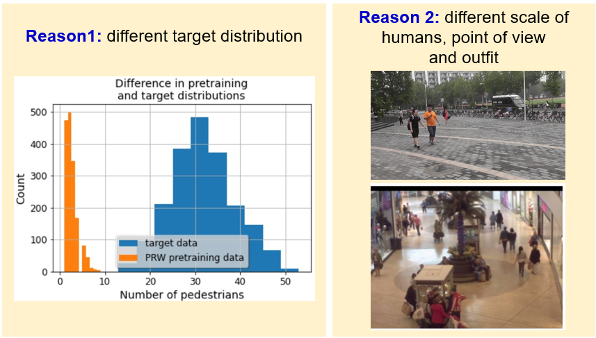
We took two random subsamples of the dataset - of 842 and 1637 images. The subsamples were used at the pre-training stage. During the procedure, the pre-training and the training share same hyperparameters, except for the number of epochs (see the image below). However, this experiment did not improve the generalization capabilities. As you see from the learning curves below, using the PRW data allows the model to start with considerably lower MAE loss values. However, all learning curves (including the one without pre-training) converge to roughly same values. Therefore, we do not include the PRW pre-training into our final solution.

The reasons, why the pre-training did not boost the model’s performance include several factors:
-
Different distribution of target variable (number of pedestrians). In the PRW dataset, the distribution is highly skewed, with the mode of roughly 3-4 people. Our target distribution, however, is bell-shaped, with a mean of around 32 pedestrians (look at the image below)
-
Difference in the poing of view, scale of humans, and even the outfit
Using advanced pre-training algorithm
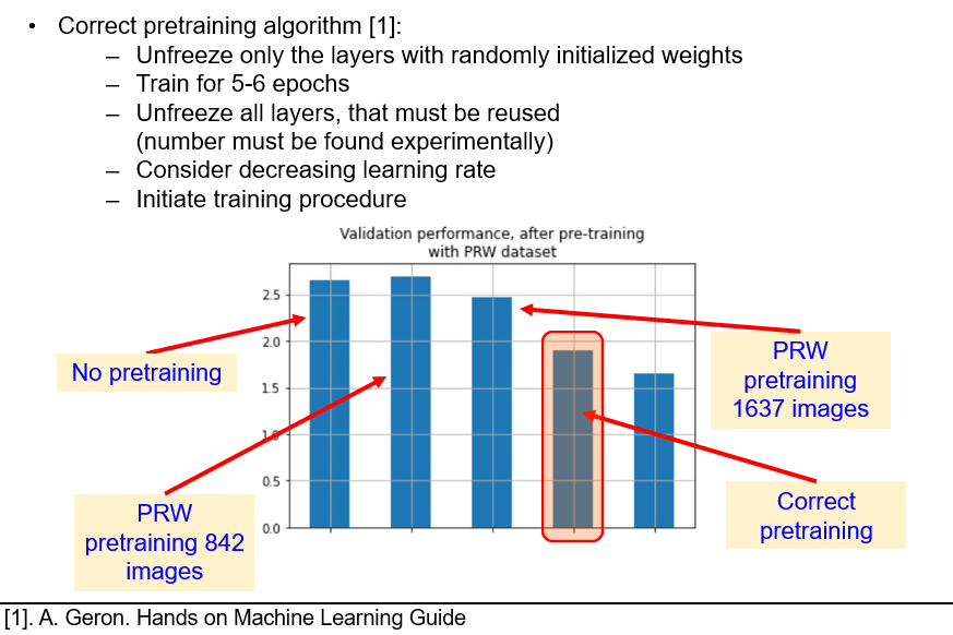
In his book, Aurelien Geron shares a correct pre-training procedure. In fact, when we utilize transfer learning approach, we append the pre-trained feature extractor with the layers, that have the randomly initialized weights. Therefore, the first gradient updates will be larger. These updates, when back-propagated, can override the knowledge, hardwired into the weights of the feature extractor during the pre-training step. To address this issure, Aurelien Geron suggests the algorithm, that is described in the image below.
Notice, how using the correct pre-training procedure gives us even better results, than using additional data! This is the first experiment, when we dropped the validation MAE below 2.0. Thus, we definitely include this algorithm into our final solution.
Final solution and a test report
Our final solution includes the Xception architecture, with the ELU activation functions (instead of the baseline-level ReLU), a deeper classification block, and the pre-training algorithm of A.Geron. You can see the training hyperparameters listed in the table below.
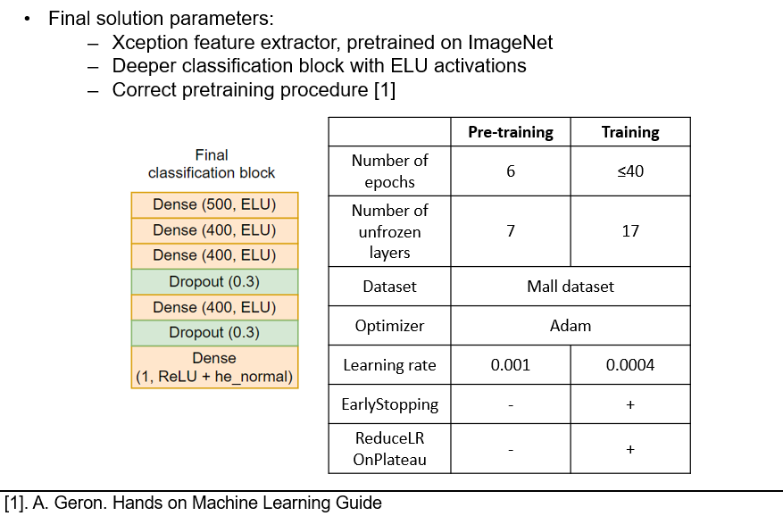
The final solution achieves 1.63 validation MAE error, which is twice as much better, compared to the regression-based approach of Chen et al.. After validating the model, it is time to try it on the test data. From the image below, we see, that the test result of 1.64 MAE is comparable with 1.63 MAE on validation, thus we have not overfit the validation set.
This is the final solution to the problem of predicting the crowd numerosity. Thank you for your attention!