Introduction

Hello there!

This article is devoted to my project, available on github. We will use popular CNN architectures to diagnose Covid 19 disease, based on X-ray lung images.

We will cover following topics:

Type II mistake, as a performance metrics
Training CNN architectures from scratch, achieving result, comparable with the research works
Comparing performance of several architectures (custom CNN, AlexNet, VGG16 and VGG19) with respect to the task of Covid 19 diagnosis
Adaptive histogram equalization methods, as a way to enhance contrast of X-ray images

Let’s get started!

Alternative methods for Covid 19 diagnosis

Nowadays, the adopted invasive testing method is a polymerase chain reaction test (PCR). Unfortunately, according to sociological research, the test has many weaknesses, when not taken at clinic:

First, as a nasal invasive test, its result depends on the sample quality. Because the procedure might not feel comfortable, poor quality of the nasal samples leads to incorrect results
Second, when samples are transported to a hospital for further testing, biological samples degradation can cause incorrect diagnosis
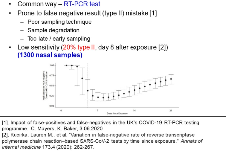
Last, PCR testing, especially in non-laboratory conditions, is characterized with low sensitivity and proneness to type II mistakes. Based on exploring 1300 nasal samples, Kucirka et al. found, that on the 7th day of exposure, at best there is a 24% probability of labelling a patient healthy, while he is COVID infected (refer to the picture below).

These findings pushed the community for finding alternative diagnosis methods. One of the alternatives is a screening method. In the image below, two variations of screening are presented – computer tomography axial CT and front chest X-ray image.

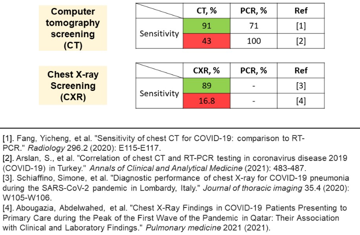
Unfortunately, the problem encountered is largely contradictory research results. As regards CT method, the reported sensitivity varies from upsetting 43% to 91%. Same applies to CXR results, where the range is even wider. An explanation for the discrepancy between results is a sampling technique. Success of screening methods largely depends on the sample of patients and stage of disease exposure. Screening methods fail on mild stages of disease, and so does the PCR test, during the first days.

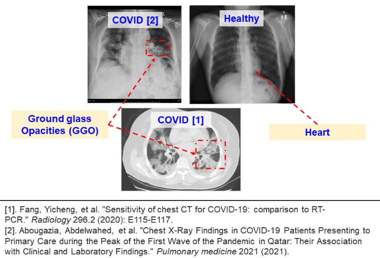
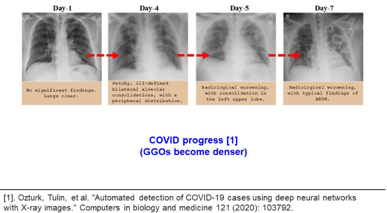
Despite the results for CT and CXR contradict each other, all authors agree about the capacity of screening methods for COVID diagnosis. The image below illustrates the ground glass opacities (GGO), reported in many related works. The GGO structures are observed both in CXR and CT methods. Moreover, the GGO structures expand with disease development.

In another research, Oztruk et al. demonstrate how the pathological structures evolve inside human lungs. This shows the potential of screening methods as an alternative for PCR testing (please refer to the image below).

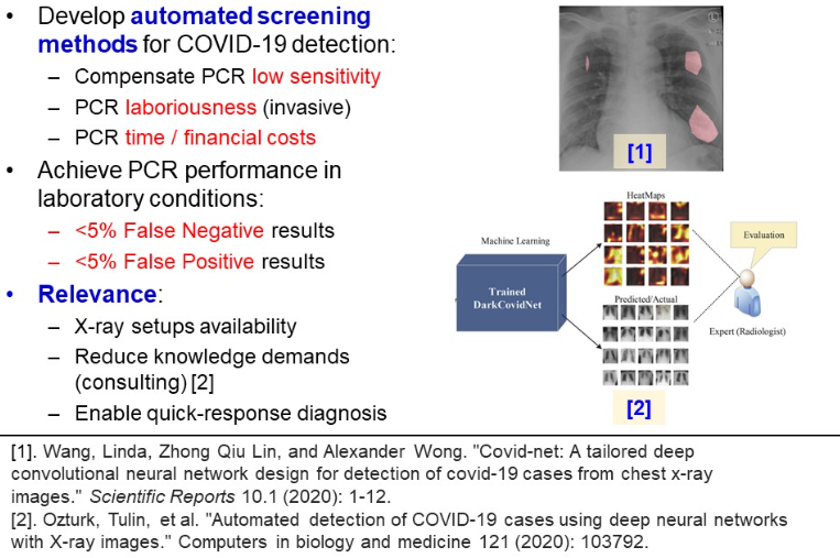
Unfortunately, the analysis of CXR images demands time costs and radiological expertise. This is why a novel approach is to take advantage of CNN models, capable of recognizing pathological GGO patterns. Deploying a machine learning classifier will compensate for PCR low sensitivity, laboriousness, time and financial costs. It will reduce necessary workforce in hospitals, necessary for conducting PCR testing. Also, this model can serve as a consulting system, giving a human last word, but providing heatmaps of the relevant regions. According to the previous research, clinical demands for PCR testing is a low percentage of false positive and false negative results. This is desirable to achieve for a machine learning model.

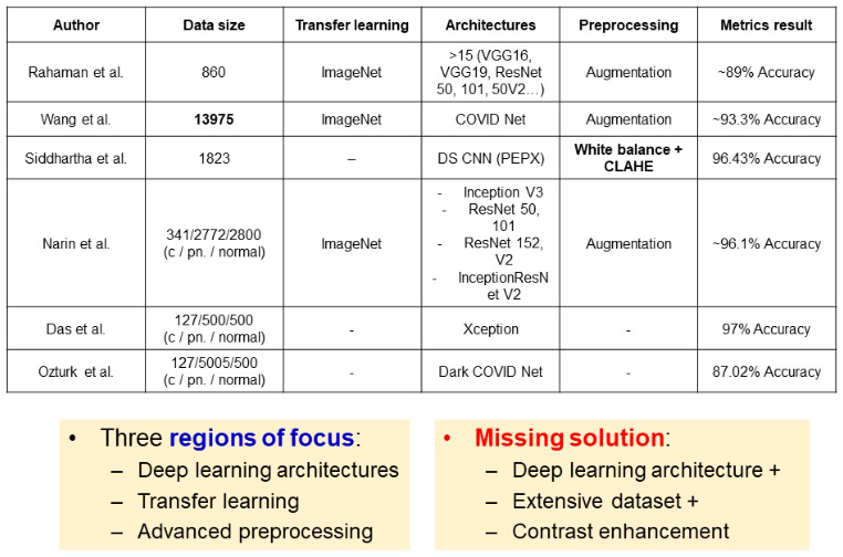
Numerous architectures and approaches have been considered. Rahaman et al. examined wide range of architectures, however used small dataset of 860 images. The largest dataset so far was used in the study of Wang, and they achieved a classification accuracy of 93.3%. Siddhartha et al. focused on contrast enhancement techniques, which allowed for 96% metrics, despite the small dataset of 1823 images. In the study of Narin et al., an imbalanced dataset was used, with wide range of deep architectures. Narin et al., as well as many others, take advantage of transfer learning with pre-training models on ImageNet dataset. Some authors like Wang and Ozturk focus on tailoring special architectures for covid classification.

Overall, authors prioritize advanced architectures, or preprocessing techniques, or large datasets. A solution was missing, which will embrace deep architectures, large data and contrast enhancement techniques.

Experiment scheme

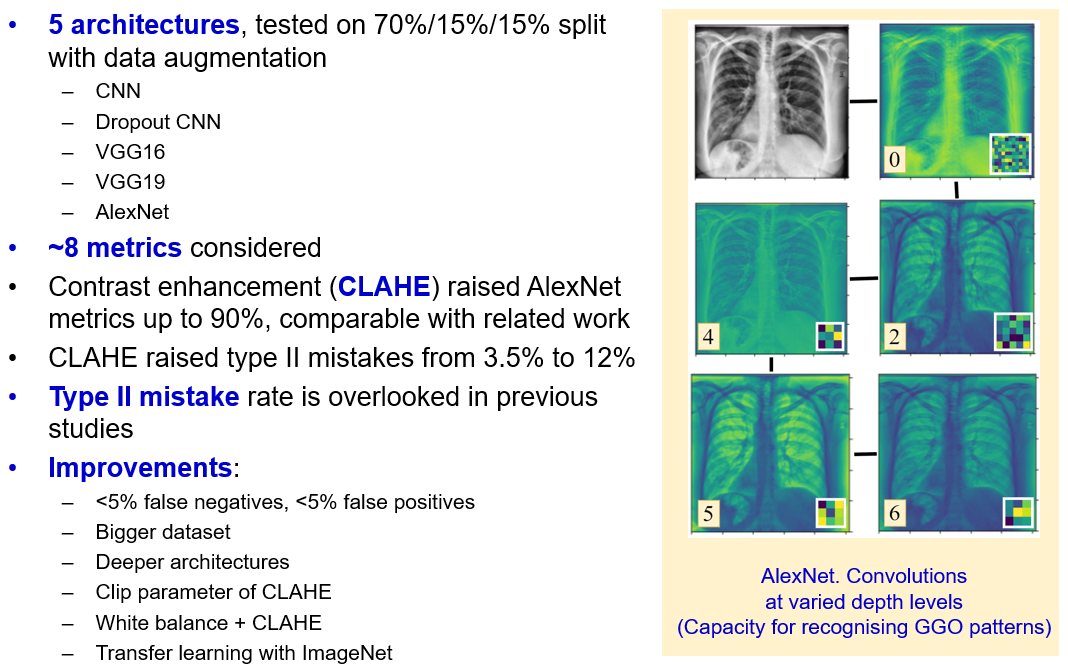
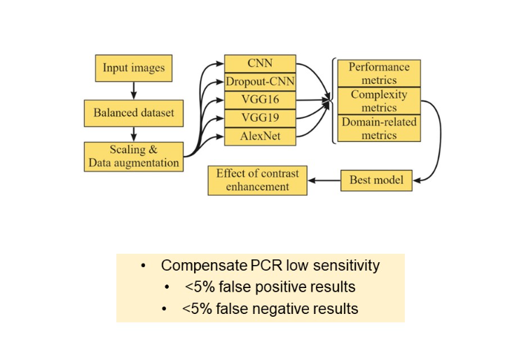
In the following section, we test five architectures:

Custom “vanilla” CNN
“Vanilla” CNN with dropout layers
VGG 16
VGG 19
AlexNet

Then, we compare models not only by performance metrics, but by complexity and their proneness to type II mistake, which is a domain related metric. On the best model, an effect of contrast enhancement techniques is studied. The main goal so far is to develop a classifier, which compensates PCR low sensitivity and achieves the PCR laboratory score of 5% false positive and 5% false negative results.

Dataset

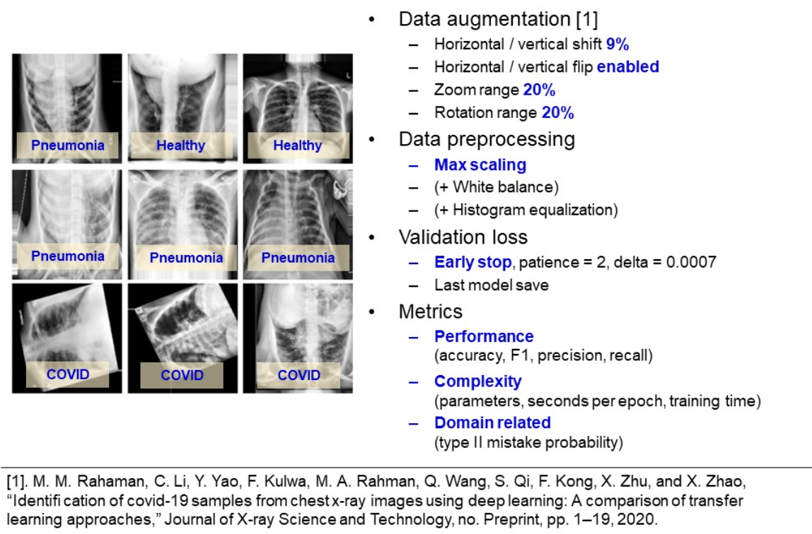
The available data consists of 4575 chest X-ray images (have a look at the example in the image below). The dataset is split into train, validation and test sets with proportion of 70, 15, 15 percent respectively. Among each dataset, the images were uniformly randomly distributed. The balance of classes gives credibility to such metrics as accuracy, precision, recall.

From visual inspection of the dataset, one concludes that the images are rotated, flipped and squeezed. Hence, for greater generalization ability, we apply the data augmentation techniques with shifting, flipping, zooming and rotating the images.

To save computational time when selecting a baseline model, initially only max–scaling is used as a preprocessing step. To prevent overfitting, a kernel regularization is used, in addition to early stopping. We monitor minimum of validation loss with a patience of two epochs. Only the last model is saved (e.g. the weights after the last epoch, but not the weights, corresponding to the best validation performance).

Models are compared based on standard classification metrics with macro averaging. Also, we account for the number of trainable parameters and seconds per epoch, as additional complexity metrics. Finally, it is a risk to label a COVID-infected person as healthy. This is what is called a type-II mistake, and used as a discriminative metric to select the best model.

Learning summary

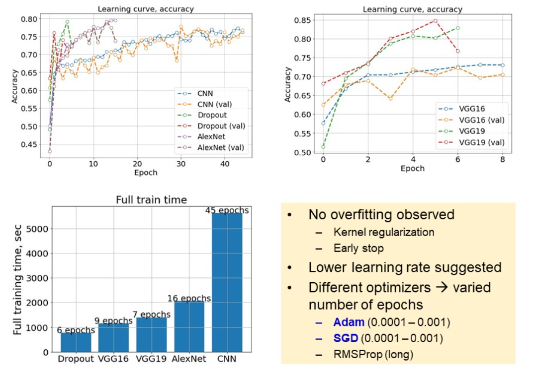
An image below represents a learning summary. Two graphs above illustrate learning curves for the considered models. Kernel regularization helped to prevent overfitting, even for CNN at more than 40 epochs of training. From the slightly unstable curves we conclude, that a lower learning rate is suggested. Overall, chosen optimizers and learning rates varied between models, which led to different number of epochs. Also, from learning curves we see, that deeper models, like VGG19 and AlexNet, have capacity for achieving better metrics, as their learning curves are more steep.

Metrics comparison

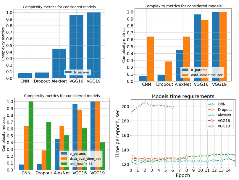
After training the models, we proceed to complexity comparison, in terms of trainable parameters. In this study, we cover a wide range of complexities. While the largest VGG19 is taken for 100%, CNN corresponds to less than 10% of VGG19 trainable parameters.

One of the charts below compares the time, necessary for each model to accomplish an epoch. We can see a large gap between the largest, and the rest of the models. VGG19 took 53% more time to accomplish an epoch. This is why, using more complex models is worthy, if and only if they give substantial gain to the model performance. At this point, we select AlexNet, as the optimal model of average complexity and evaluation time. The next step is to compare models on the test set.

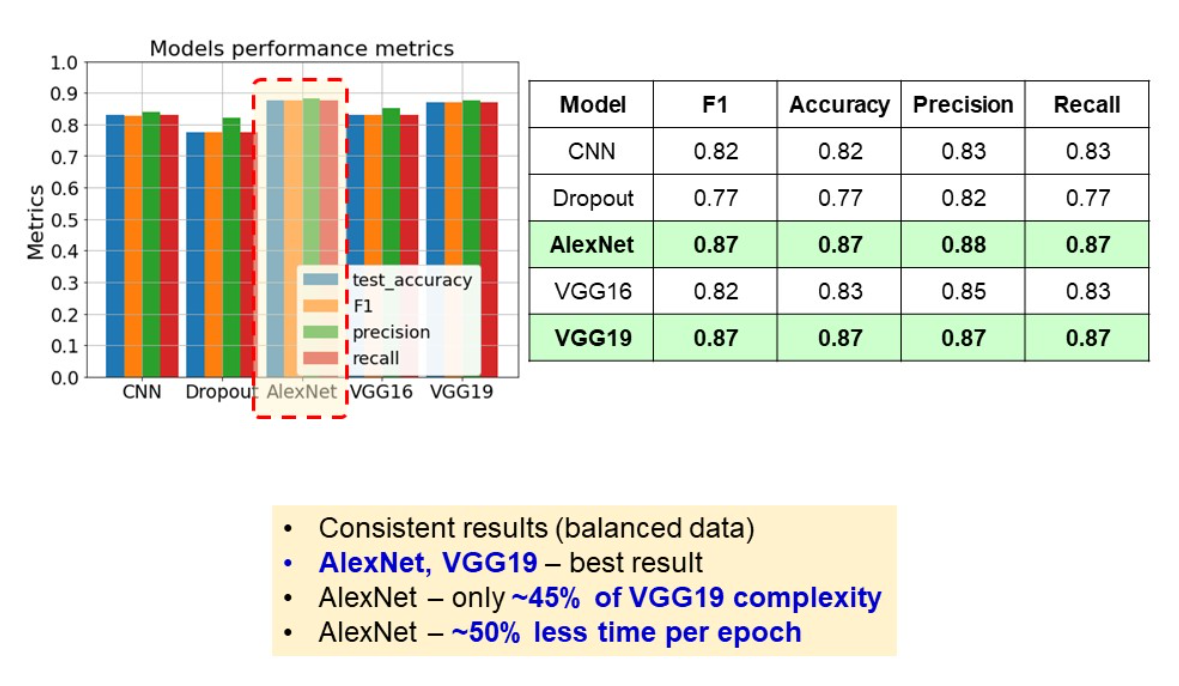
We use four classification metrics for models comparison – F1, accuracy, precision and recall. Remember, a recall is a crucial metric, as it describes the model’s ability to distinguish the infected patients from healthy. According to these metrics, we highlight AlexNet and VGG19 with the best scores achieved. However, according to the complexities, covered in previous slide, AlexNet has 45% less trainable parameters than VGG19 and requires twice as less time to accomplish an epoch.

Type II mistake probability

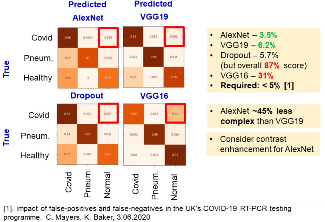
The last metric is a probability of type two mistake. Because it is not as critical to label a healthy to have COVID, as to claim a COVID-infected person as healthy.

Confusion matrices in the figure below were built based on the test predictions. One has to focus on the right upper square of the matrix. We see, that AlexNet, VGG19 and Dropout give result of around 5%. However, Dropout model underperformed in terms of accuracy, precision. Because AlexNet is a lightweight model, which gives one of the best performance metrics and one of the least type II mistakes rate, we claim it to be the best model and study the effect of contrast enhancement in the next chapter.

Effect of contrast enhancement

In the related works, an adopted contrast enhancement technique is called contrast limited adaptive histogram equalization (CLAHE). This method allowed Siddhartha et al. to achieve roughly 96% accuracy. According to the images below, one could see that this technique indeed highlights the bones and ground glass opacities.

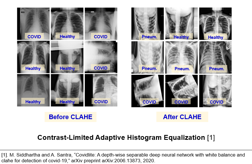
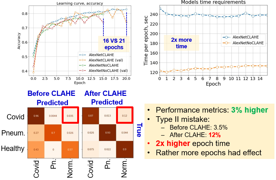
Therefore, CLAHE algorithm was applied as a preprocessing step, after resizing and max-scaling the images. However, here we faced contradictory results. First, from the learning curves (image below) it is seen, that models were trained during different number of epochs. It is possible to conclude, that it is the larger number of epochs, which affected the model performance, but not the preprocessing.

Second, learning with histogram equalisation takes twice as much time to accomplish one epoch (image below). Therefore, before applying advanced techniques for preprocessing, it made sense to start with only scaling and choose a baseline model.

Third, from the confusion matrix we can see, that AlexNet with CLAHE and higher number of epochs performed overall much better, in terms of false positives and false negatives for pneumonia-healthy pairs and type I mistakes. However, the probability of type II mistakes increased up to 12%. Overall, the contribution of histogram equalization is still debatable. We suppose, that it is the larger number of epochs which influenced the performance.

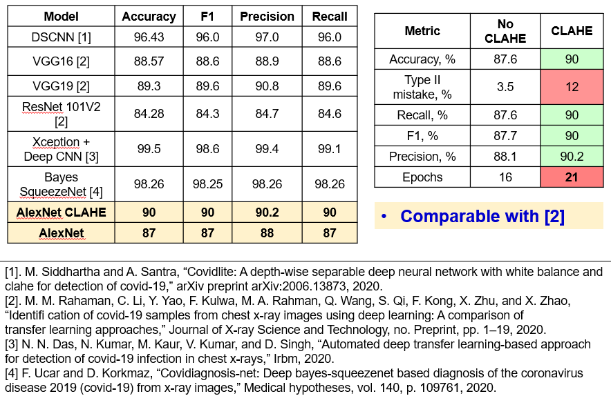
In the image below (right table), we compare results before and after CLAHE preprocessing. We see, that the probability of type II misclassifications is the only metric which increased. Otherwise, larger number of epochs and preprocessing gave 3% gain for other metrics. Also, a table on the left compares suggested solution with the state-of-the art from related research. It is seen, that the results are comparable with ResNet101V2, VGG16 and VGG19 from the work of Ramahan. However, the model fails to compete larger models, trained with ImageNet dataset, and particular models like depth-wise separable CNN, Bayes SqueezeNet, Xception.

Conclusion

In this work, five deep learning architectures were studied, to explore the CNN capability for recognizing the ground glass opacities inside the patients’ lungs. A standard split with 70/15/15 is used, together with data augmentation and max-scaling.

Based on eight metrics (performance, complexity and domain-related), AlexNet model appeared to be the “golden middle” with average number of parameters, training time, and performance metrics. Contrast enhancement techniques raised the metrics of AlexNet up to 90%, however raised the proneness to type II mistakes as well.

The important conclusion is that the type II misclassifications is an important metric, which allows to easily discriminate between appropriate and poor performance. However, in the previous studies, authors were rather focused on standard metrics, such as accuracy, F1, precision and recall. This should not be overlooked, while developing a system for disease diagnosis.

A possible improvement of this work is a complex solution, which embraces all components:

Bigger dataset
Deeper architectures (Xception, ResNet)
Finding the optimal clip hyperparameter of CLAHE preprocessing
Adding white balance, to compensate for light scarcity on CXR images
Use pretrained models

← Previous Post Next Post →