Introduction

Hello there!

This article is devoted to my project, available on github. We will see how Deep Belief Networks (DBN) learn visual concepts and study how Restricted Bolzmann Machines (RBM) capture statistical patterns from visual data.

In a rapidly developing sphere of machine learning and artificial intelligence, a significant part of research corresponds to unsupervised learning models. Learning without answers allows models to perform feature extraction, making them more resembling of “natural” learning process. In this work, we take advantage of a deep belief network (DBN), used for capturing hidden data representations, based on letter images from EMNIST dataset. Using DBN model allowed for analysis of hidden data representations through visualising neuron receptive fields at several depths. Moreover, linear read-outs are performed, to compare DBN classification performance with a supervised feed forward neural network (FFNN).

To assess a DBN’s ability to grasp similar visual concepts, an analysis with hierarchical clustering methods and confusion matrices is performed. Finally, both DBN and FFNN robustness are validated, providing gaussian noise, salt & pepper noise, and adversarial attacks.

Data

Model training is based on letters, provided by EMNIST dataset. Each data instance represents a greyscale-value image of 28 × 28 pixels, like in figure below.

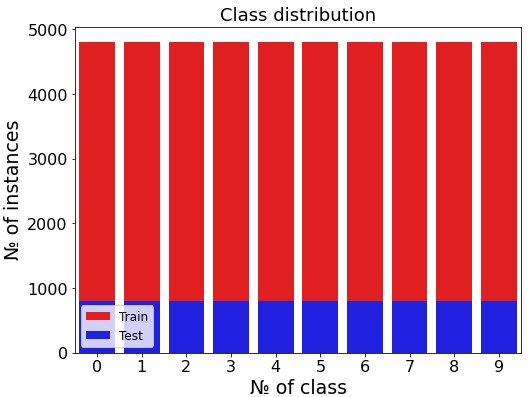
For this study, we limited the whole dataset with ten classes and 4800 images for each class. Thus, both models are trained on a set of 48000 images, while the accuracy is reported based on 8000 unseen data instances.

Before training models, it was made sure that the class distribution is uniform for both train and validation sets. This proves accuracy to be a valid metrics for models comparison (image below).

Preprocessing procedure includes max-scaling the data, by dividing the images greyscale value by the maximum of 255.

Model, architecture

In this work, two types of architectures are presented - a shallow DBN model with 500 hidden units, versus a deep belief network with two hidden layers of 500 units each. One needs to choose an FFNN architecture accordingly with the chosen DBN structure. Hence, the presented FFNN model has one hidden layer of 500 neurons, and 784 input neurons, representing flattened pixels of an input image.

In addition, several perceptrons were trained for multi-classification task, with DBN hidden layers as input. In latter parts, FFNN performance will be compared with perceptrons, trained on DBN hidden representations, instead of raw images.

Training and validating method

For comparison purposes, a Feed Forward Neural Network (FFNN) was trained during approximately the same time as the shallow DBN model. This is why number of training epochs varies between two types of architectures - 1500 and 120 epochs perceptron and FFNN model respectively. Since the datasets are balanced, we select accuracy, as a metric to compare models performance.

Receptive fields visualization

A figure below presents neurons receptive fields of a deep belief network. Each receptive field represents a layer of weight matrix W, projected at two dimensional space of 28 × 28 pixels. Thus, a greyscale value highlights the neurons connection strength. The higher the greyscale value, the more important a certain regiou (visual concept) of the image is. In two images, we present the neurons receptive fields of the first and the second hidden layer.

The receptive fields clearly visualize, how an unsupervised model captures more specific details with deeper hidden layers. While the first layer receptive fields are essentially greyish, (not specified), deeper layers focus on particular types of letters features, as it is demonstrated by bright dots and lines on contrast receptive fields.

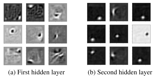
Thus, deeper level receptive fields indicate a separation of responsibility between neurons. Certain groups of hidden units are responsible for particular features detection.

Internal representations clustering

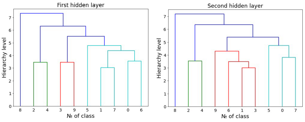
In order to understand, if an unsupervised model was able to capture similar visual features, one can calculate mean hidden representations, corresponding to each class. Afterwards, an hierarchical clustering algorithm has to be applied to mean representations, to evaluate their similarity. Please refer to an image below, to see the example.

What you will see is a dendrogram. It summarizes similarities, that the model has learnt from the visual data. For example, it finds, that classes two and four, three and nine, one and seven, and zero with six are very similar (according to the left dendrogram). As the knowledge representations of deeper layers change, they find similarities between different pairs of classes.

Let us pair images, according to the similarities, discovered by the model, and visually assess, if they are really similar? 👇

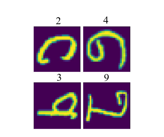
The answer is – yes, indeed, from visual analysis one can conclude, that unsupervised model successfully encodes similarity of visual concepts.

Linear read-out performance

In this chapter, we report models performance on unseen validation data. We perform linear read-out, which is a technique, that uses internal representations of hidden DBN layers as input data for perceptrons, trained for multiclassification problem. In this way, the input for the final model is no longer raw, training data, but the representations of knowledge, captured by deep belief network. In theory, it makes the learning process easier, as the raw data was already pre-processed, to discover most meaningful features of input images.

In this chapter, we compare performance of perceptrons, trained on hidden representations, with FFNN model, trained on raw images. Thus, hidden layer of FFNN network is both responsible for feature extraction, as well as for tuning for the multiclassification task.

A figure below summarizes accuracies on the validation dataset. It clearly demonstrates benefits of learning from data with pre-extracted features, generated by unsupervised models. Linear read-outs outperform FFNN model by around 10%, with an accuracy above 80% on unseen data.

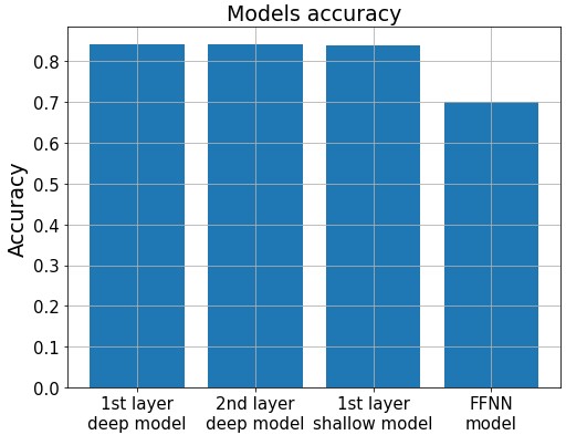
Moreover, internal representations are favored over raw images, since they serve as “shared” data for multiple tasks (e.g. letter and digit recognition). Thus, using shared representation is beneficial, because one can flexibly readjust model for another task, instead of retraining model from scratch.

Noise robustness

Let us compare models’ performance with unseen data, distorted by random noise insertions. Two types of noise are introduced. Figure below illustrates distortions, imposed by Salt & Pepper and Gaussian random noise.

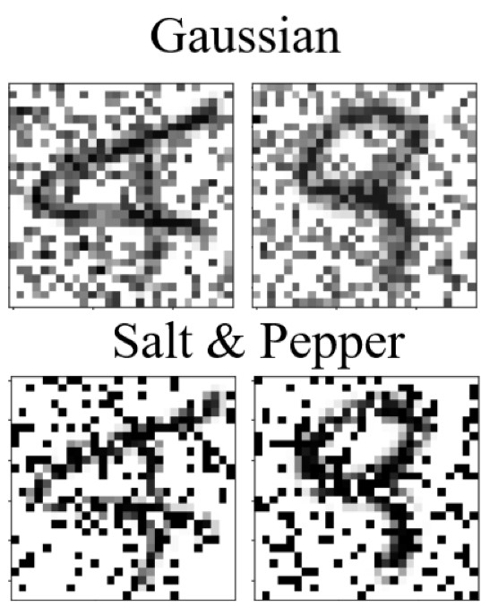
For noise coverage, ranged from 0% (original image) to 50%, we perform accuracy computation on the unseen validation data. Figures 9 and 10 below report models’ accuracies on the test set.

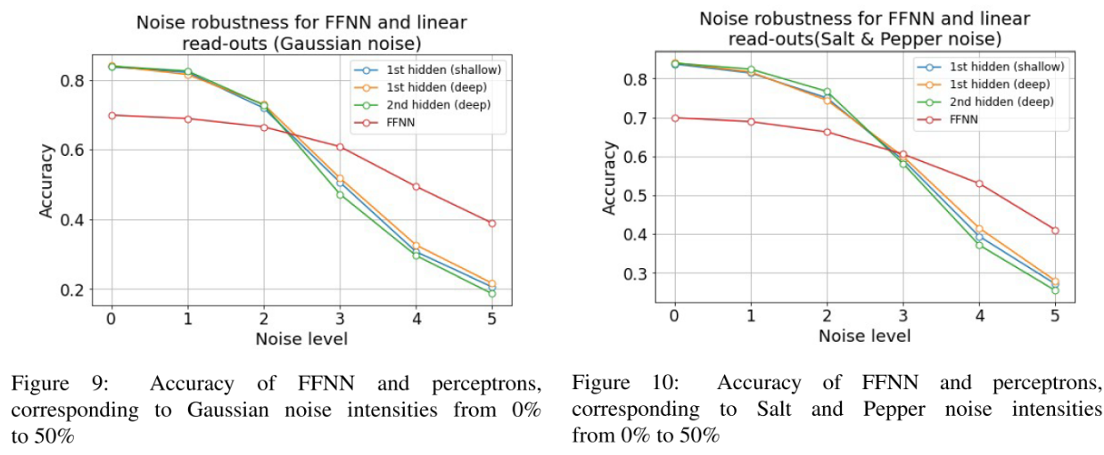
In summary, perceptrons, learned on hidden representations of various depths, outperform FFNN model for noise intensities up to 30%. In addition, models behaviour was consistent for both Gaussian and Salt and Pepper noise.

Adversarial attacks

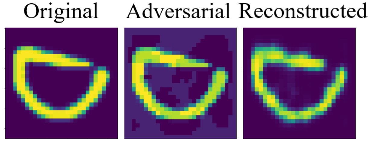
One beneficial trait of DBN model is the capability for data reconstruction, which is essential for adversarial attacks. For instance, a figure below demonstrates that, by adding specific noise, accounting for loss function gradient, it is feasible to negatively affect model’s predictions.

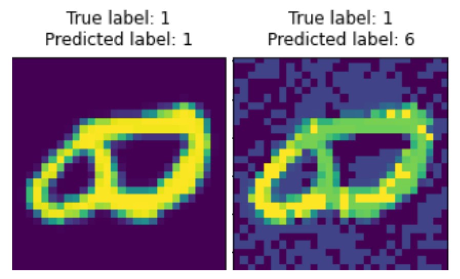
However, DBN capacity for reconstruction allows the this model to stay robust against adversarial examples. For instance, after two reconstruction steps, performed by shallow DBN, resulting image is almost free of adversarial distortions.

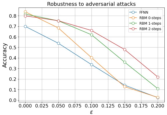
To evaluate DBN robustness against adversarial samples, its accuracy was assessed on the test set, exposed to attack intensities ϵ ranged from 0 to 2.25, where ϵ stands for gradient multiplication coefficient. Thus, a plot below emphasizes importance of reconstruction. Compared to FFNN model with the steepest accuracy decline, two reconstruction steps allow perceptrons to maintain accuracy of around 70% for weak attacks with ϵ less than 0.05.

Confusion matrix analysis

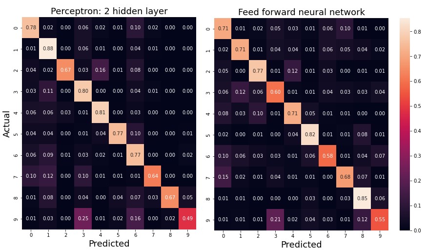
Confusion matrices allow to understand the nature of misclassifications and identify similar alphabet symbols.

Along the main axes of two confusion matrices below, the underperformance for certain classes is clear. For instance, 18% of FFNN misclassifications account for classes nine and three, which are actually visually similar, as you can make sure from the images.

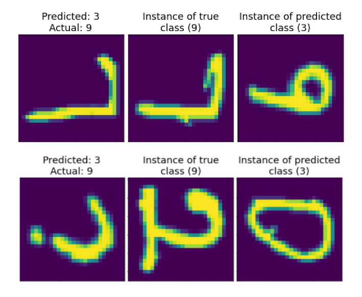
All confusion matrices exhibit the same pattern. For instance, also the model, learned from internal representations of the first hidden layer, in 17% of cases labels instances of class nine as letters, corresponding to class three. One of possible explanations for underperforming of models is a greater variety of written letters, as opposed to digits in MNIST dataset. EMNIST letters encapsulate both upper-case and lower-case letters as instances, corresponding to the same class, which ensures a greater statistical variety.

Conclusion

In this study, we compared visual concept learning, implemented by deep belief network and feed forward neural network. Neuron receptive fields visualizations emphasized how DBN units infer visual features. Mean hidden representations clustering proves DBN ability for capturing similarities between different classes. Finally, perceptrons, learned on internal representations, demonstrate higher accuracy (80%), as opposed to feed forward neural network with 70% accuracy on the validation set. Moreover, DBN model exhibits highter robustness to two types of noise and adversarial attacks. Confusion matrix analysis revealed that mostly, all studied models misclassify visually similar instances.

---